Quick Start and Tutorial

• Examples are in the demos subdirectory.

• Dataguzzler-Python configurations are written in Python and saved with the .dgp filename extension. Configure your text editor to interpret .dgp files as Python to help with indentation and syntax highlighting.

• Dataguzzler-Python configuration include files are normally stored as part of a Python package, written in Python and saved with the .dgi filename extension. Configure your text editor to interpret .dgi files as Python to help with indentation and syntax highlighting.

Because Dataguzzler-Python is a command line tool, the first step to running Dataguzzler-Python is usually opening up a suitable terminal or command prompt window. If you are using Anaconda on Windows, this means opening an Anaconda Prompt or Anaconda PowerShell Prompt from the start menu.

In addition, your terminal or command prompt needs to be configured to use a Python environment that has Dataguzzler-Python installed. If you are using Anaconda, environment selection is performed with conda activate, for example if you followed the Anaconda environment creation instructions in the installation section,

conda activate SNDE

Dataguzzler-Python is run from the command line by giving it the name of a configuration file as its first parameter. The simplest example is in configdemo.dgp, which defines a dummy class that pretends to interact with hardware, and then instantiates the class into a Dataguzzler-Python module.

From the Dataguzzler-Python demos directory:

dataguzzler-python configdemo.dgp

The response represents the dummy hardware initialization and an interactive Dataguzzler-Python REPL (Read Evaluate Print Loop) prompt:

Init the hardware
dgpy>

The Dataguzzler-Python REPL is similar to the standard Python REPL but with a few minor differences:

• It is designed to support multiple parallel loops representing control from different sources (such as an interactive terminal at the same time as a script).

• As of this writing it does not (yet) support multi-line commands.

• It always prints the expression value (even if None)

• The response starts with a fixed size header to simplify automated interpretation.

• Assignment statements are treated as having a value.

If you look at configdemo.dgp you will see that it defines a class DemoClass and instantiates it as the object Demo. Since DemoClass uses dgpy.Module as its metaclass, its instances (such as Demo) are Dataguzzler-Python modules. That gives them special interactive characteristics (as well as functionality to manage multithreading).

If you type Demo and press <Enter>, Dataguzzler-Python will respond with a header and the object’s representation (Python repr()):

dgpy> Demo
200 000000000050 <dgpy_config.DemoClass object at 0x7fb583f33b20>
dgpy>

You can issue commands such as calling the object methods .read() and .write():

dgpy> Demo.read()
read from the hardware
200 000000000006 None
dgpy> Demo.write()
Write to the hardware
200 000000000006 None
dgpy>

For a module that controlled actual hardware, the read method might return a value and the write method might accept a parameter to write, instead of both just printing to the console. Note that print functions like those in the class always output to the main console, whereas the responses (both None) are returned to whichever connection issued the command.

Oftentimes we don’t remember the names of methods so it is useful to be able to introspect an object to see what we might do with it. Some such functionality is built into Python, such as the dir() function:

dgpy> dir(Demo)
200 000000000452 ['__call__', '__class__', '__delattr__', '__dict__', '__dir__', '__doc__', '__eq__', '__format__', '__ge__', '__getattribute__', '__gt__', '__hash__', '__init__', '__init_subclass__', '__le__', '__lt__', '__module__', '__ne__', '__new__', '__reduce__', '__reduce_ex__', '__repr__', '__setattr__', '__sizeof__', '__str__', '__subclasshook__', '__weakref__', '_dgpy_compatible', '_dgpy_contextlock', '_dgpy_contextname', 'help', 'read', 'who', 'write']
dgpy>

However, the output of dir() is polluted by a lot of internal-use-only attributes that you don’t usually want to see. Therefore Dataguzzler-Python provides a function who() that hides the irrelevancies:

dgpy> who(Demo)
200 000000000019 ['read', 'write']
dgpy>

The who() function can be similarly called without a parameter to get a cleaned-up listing of accessible variables. The who() function returns both connection-local and global variables versus dir() without a parameter lists only connection-local variables. You can also pass Dataguzzler-Python modules and other objects to the Python help() function to view built-in help on the object (please note that as of this writing, help does not work properly except on the main console).

For convenience and to reduce typing, .who(), .dir(), and .help() methods are automatically added to all Dataguzzler-Python modules so you don’t have move the cursor all the way to the front of the line to get more information, e.g.

dgpy> Demo.who()
200 000000000019 ['read', 'write']
dgpy>

A more sophisticated example of instrumentation control is included in shutter_demo.dgp. The hardware in this example is write-only and the example is configured by default to use a loopback port instead of a physical serial port so that you can try it without requiring hardware (if you issue way too many commands it may freeze if the loopback buffer overflows, since nothing is emptying the written commands). Try:

$ dataguzzler-python shutter_demo.dgp
dataguzzler-python shutter demo
-------------------------------
You can control the shutter with: shutter.status="OPEN"
or shutter.status="CLOSED"

You can query the shutter with: shutter

Sometimes the shutter will be MOVING because it is slow

You can explore the variables, objects, and class structure
with e.g. who() or shutter.who() or shutter.help()
dgpy>

Try opening the shutter with shutter.status="OPEN" and then querying it with just shutter.status. If you are quick you will see the status as MOVING before it reaches the final state of OPEN. This example is a good context for practicing introspection with dir(), who(), and help().

In this example the primary module you interact with is shutter which is an instance of the servoshutter class defined in servoshutter.py. The servoshutter class does not connect to hardware directly, but instead builds on another module, servocont, which is an instance of pololu_rs232servocontroller that uses the pySerial library to talk to the actually hardware (or a dummy loopback port).

This example also illustrates both the merits of Dataguzzler-Python’s multithreaded architecture and how Dataguzzler-Python dramatically simplifies the code you have to write to do safe multithreading. The example can accommodate simultaneous commands and queries from multiple connections (such as the console and one or more network links) without deadlocks or problematic race conditions.

Each Dataguzzler-Python module has a unique context, and only one thread can be active in that context at a time. The dgpy.Module metaclass modifies all methods of the module to switch into and out of the context on entry and exit respectively. Thus most module methods run atomically and you don’t have to worry about race conditions where methods might interfere or the same method might be running twice.

The main exception is when calling other modules. Calling another module switches the context and thus the state of this module might change during the call to the other module, creating a possible race condition. However, these sorts of race conditions are usually benign as they tend to come up when you give simultaneous contradictory commands. Nevertheless, some thought may be needed to mitigate rare cases where conflicting commands or inconsistent internal state might cause physical damage (a future version of Dataguzzler-Python may support more sophisticated protocols for avoiding such race conditions).

A second exception to the atomic execution of module methods illustrates the power of the Dataguzzler-Python architecture. The shutter object has a .wait() method (try it!) to wait until the last move has had a chance to complete. Waiting is problematic in single-threaded data acquisition because you either lock out the primary thread for the duration of the wait, or you have to have some means to return to the main loop and get a notification and callback later once the event of interest has occured. The servoshutter.wait() method illustrates use of the Dataguzzler-Python RunUnprotected() function to wait while dropping the module context (so other commands can be processed during the wait). The net result is simpler code with far fewer worries about locking.

It is architecturally a good idea to separate out low level mechanisms from higher-level sequencing and policy, and this example illustrates how that can be done. The pololu_rs232servocontroller class (implemented in pololu_rs232servocontroller.py) provides a low level abstraction that represents the underlying servo controller. Because it is a module it has its own context, and therefore methods will run atomically except for calls to other modules, RunUnprotected(), etc. ensuring that synchronous (command-reponse) interaction with the device will not be interrupted. The high level servoshutter can be thought of as a virtual instrument build upon the lower-level pololu_rs232servocontroller hardware module.

Using the SpatialNDE2 Recording Database

The SpatialNDE2 recording database provides a facility to store array data, to perform transformations such as accumulating data into larger chunks or performing mathematical operations, and to maintain a coherent picture of the measured state of an experiment at any given instant. The SpatialNDE2 recording database also provides a live, interactive viewer for visualizing the data, as well as the ability to raytrace data onto 3D objects and to render visualizations of those objects.

In order to use the SpatialNDE2 recording database, it must be installed in the same Python installation or virtual environment as Dataguzzler-Python. You can try the very simple example configuration and .ande file loader in the demos/ directory with:

$ dataguzzler-python ande_viewer.dgp SCANINFO_EG5_singleframe.ande

You will perhaps see some information on any accelerated compute (OpenCL) devices found, and then get a dgpy> prompt and a viewer window.

SpatialNDE2 stores data in channels that are updated during transactions. Each transaction creates a new global revision which can be thought of as a snapshot of the acquired data from a particular instant in time. The value of a channel in a particular global revision is represented by a recording, which is usually a multi-dimensional array of numbers.

Once created, channels can be selected (color change) and enabled (solid dot) on the left hand side of the viewer window. The viewer window always shows the most recent global revision for which all data is ready and all processing is complete. The screenshot below illustrates viewing SCANINFO_EG5_singleframe.ande and colormapping the ss_greensinversion channel which represents results of a thermography model-based inversion of impact damage.

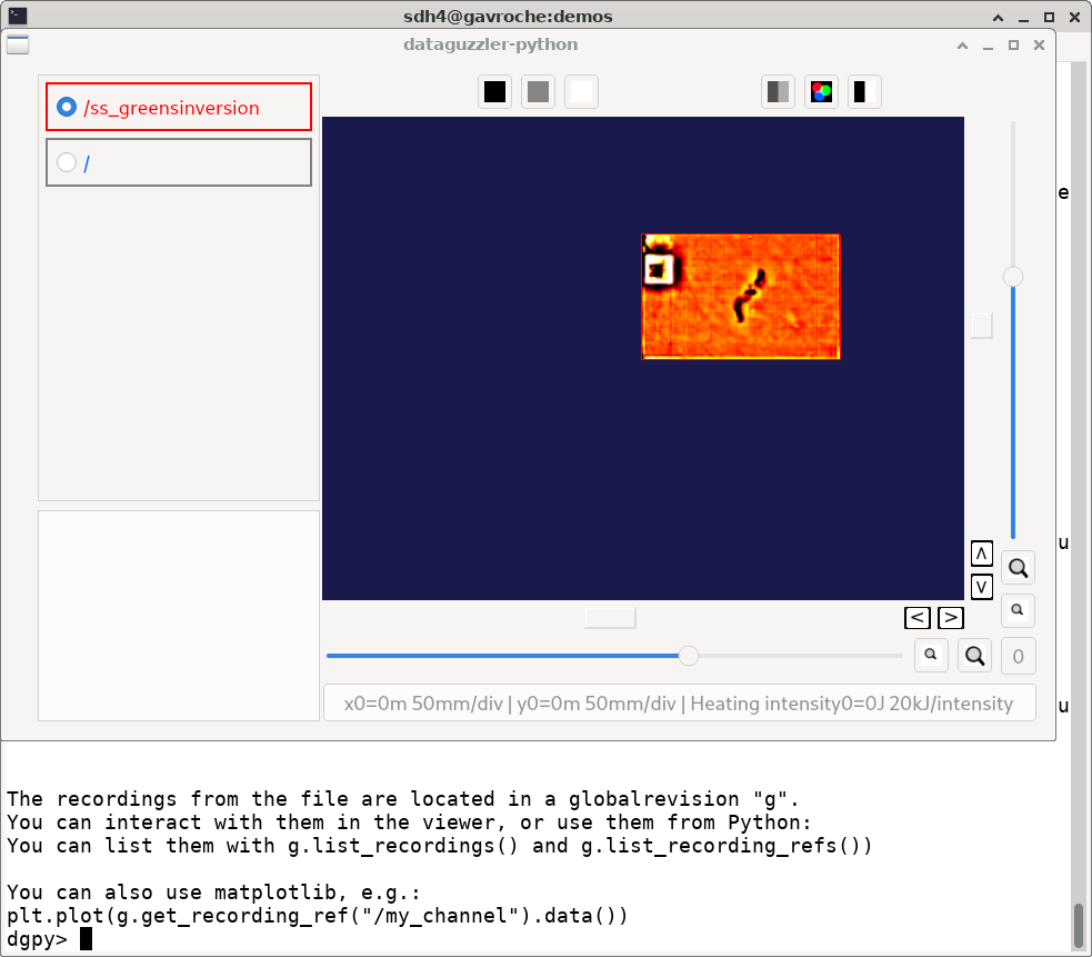
To match the screenshot you may need to reduce the default contrast (top bar icon with two gray vertical strips) and switch the colormap (red-green-blue icon).

You can also access and view the data directly. The ande_viewer.dgp configuration automatically stores the globalrevision with the loaded data in the variable g (alternatively you could obtain the latest data with g=recdb.latest_globalrev()).

You can see the different recordings that are defined with g.list_recordings()

dgpy> g.list_recordings()
200 000000000033 [
"/",
"/ss_greensinversion",
]
dgpy>

A recording itself can sometimes (rare situations) have multiple data arrays, so if we want to access data arrays we usually need to access the recording data array reference (“recording ref”) corresponding to the recording:

dgpy> r = g.get_ndarray_ref("/ss_greensinversion")
200 000000000139 <spatialnde2.ndarray_recording_ref; proxy of <Swig Object of type 'std::shared_ptr< snde::ndarray_recording_ref > *' at 0x7f44c592e540> >
dgpy>

Then we can look at the data array by calling the .data() method:

dgpy> r.data()
200 000000000629 array([[-12328.111 , -12328.111 , -12328.111 , ..., -19782.75  ,
        -19782.75  , -19782.75  ],
       [-12328.111 , -12328.111 , -12328.111 , ..., -19782.75  ,
        -19782.75  , -19782.75  ],
       [ -1005.9551,  -1005.9551,  -1005.9551, ..., -16413.162 ,
        -16413.162 , -16413.162 ],
       ...,
       [  4599.9766,   4599.9766,   4599.9766, ...,   1981.196 ,
          1981.196 ,   1981.196 ],
       [  5834.971 ,   5834.971 ,   5834.971 , ...,  -5064.434 ,
         -5064.434 ,  -5064.434 ],
       [  5834.971 ,   5834.971 ,   5834.971 , ...,  -5064.434 ,
         -5064.434 ,  -5064.434 ]], dtype=float32)
dgpy>

The metadata goes with the recording itself r.rec not the recording array reference r, and can be accessed with r.rec.metadata:

dgpy> r.rec.metadata
200 000000000141 <spatialnde2.constructible_metadata; proxy of <Swig Object of type 'std::shared_ptr< snde::constructible_metadata > *' at 0x7f44c592e600> >
dgpy>

The metadata can be printed in human readable form by converting it to a string:

dgpy> str(r.rec.metadata)
200 000000000434 r"""Coord3: STR "Depth Index"
ande_array-axis1_scale: DBLUNITS 0.0005 meters
IniVal3: DBL 0
Units3: STR "unitless"
ande_array-axis0_coord: STR "X Position"
ande_array-axis0_offset: DBLUNITS 0.000125 meters
ande_array-axis1_offset: DBLUNITS 0.000125 meters
Step3: DBL 1
ande_array-ampl_coord: STR "Heating intensity"
ande_array-ampl_units: STR "J/m^2"
ande_array-axis0_scale: DBLUNITS 0.0005 meters
ande_array-axis1_coord: STR "Y Position"
"""
dgpy>

Note the axis label and position information embedded in the metadata.

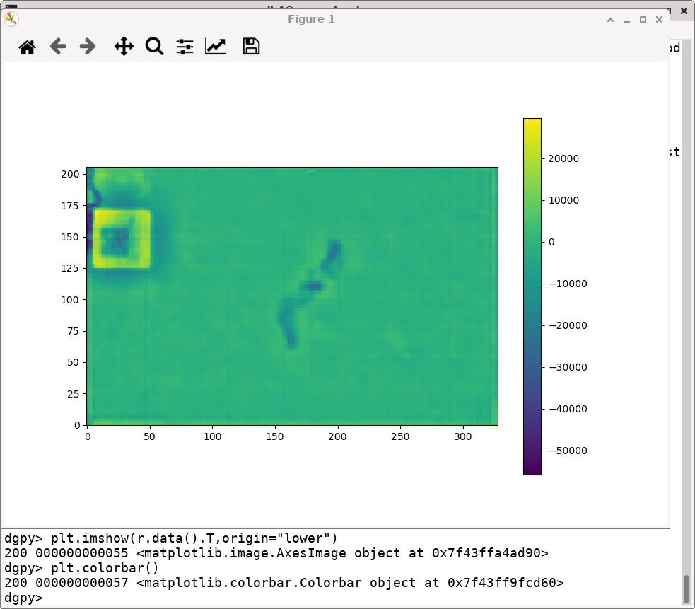
The ande_viewer.dgp Dataguzzler-Python configuration also includes support for interactive plotting with Matplotlib. This is enabled by the include(dgpy,"matplotlib.dpi") line inside ande_viewer.dgp. To new the same data in Matplotlib:

dgpy> plt.imshow(r.data().T,origin="lower")
200 000000000055 <matplotlib.image.AxesImage object at 0x7f43ffa4ad90>
dgpy>

The data is transposed because the saved file had its axes ordered (x,y) where as Matplotlib imshow expects (row, column). The origin="lower" keyword argument likewise tells Matplotlib that the origin is in the lower left, as in the SpatialNDE2 viewer. The screenshot below illustrates the loaded data plotted using Matplotlib.

You can also define new channels and recordings, but all such changes to the recording database must be performed within a transaction. To define a new channel and create a recording with an array of 32 bit floating point numbers:

transact = recdb.start_transaction();
testchan = recdb.define_channel("/test channel", "main", recdb.raw());
test_ref = snde.create_ndarray_ref(recdb,testchan,recdb.raw(),snde.SNDE_RTN_FLOAT32)
globalrev = transact.end_transaction()

The above code starts a new transaction, defines a new channel, creates a recording for that channel, and ends the transaction but does not put any data in the recording. For a particular recording database only a single transaction can be open at a time, so all other transactions will have to wait between the start_transaction() and end_transaction() lines. The actual recording is test_ref.rec and test_ref is a reference to the array within the recording.

While the above code defined a new recording, it did not provide the recording with data and mark it as “ready”, so the SpatialNDE2 library will still be waiting for data. Additional transactions can proceed after end_transaction() but the recordings added in globalrev will not display in the viewer and newer data will accumulate in memory waiting for the recording test_ref.rec to be marked as ready.

There are several possible steps to providing the test_ref recording reference with data. First, it is common to attach metadata to the recording, such as for axis information:

test_rec_metadata = snde.constructible_metadata()
test_rec_metadata.AddMetaDatum(snde.metadatum_dbl("ande_array-axis0_offset",0.0));

test_ref.rec.metadata = test_rec_metadata;
test_ref.rec.mark_metadata_done()

Second, memory needs to be allocated to store the array data:

rec_len = 1000
test_ref.allocate_storage([ rec_len ],False)

You can pass multple lengths to create a multi-dimensional array. The second parameter, which defaults to false determines the storage layout for multidimensional arrays. If false, the array will be stored with the rightmost index selecting adjacent elements (row major, C style); if true, the array will be stored with the leftmost index selecting adjacent elements (column major, Fortran style.

For programmed code it is good practice to lock an array before reading or writing it. (Array storage is managed by a storage manager in SpatialNDE2 and locking is unnecessary for interactive use almost all conditions and storage managers). For example:

locktokens = recdb.lockmgr.lock_recording_refs([
  (test_ref, True),
],False)

You provide a sequence of (recording reference, read/write) pairs where the second element is false for read and true for right. It is important to lock all recordings in a single method call because at way the locking code can ensure a consistent locking order is followed. Multiple simultaneous read locks on a given array are possible. Only one write lock can be held for a given array at a time, and no read locks can exist in parallel with that write lock. The locks will last until explicitly unlocked (snde.unlock_rwlock_token_set()) or until the containing object is destroyed. Please note that you must not call (directly or indirectly) another Dataguzzler-Python module while holding a data lock. This is because SpatialNDE2 data locks follow Dataguzzler-Python module contexts in the locking order so the context switch involved in calling another module would be a locking order violation!

You can obtain a numpy array for the recording array with the .data() method:

test_ref.data()[:] = np.sin(np.arange(rec_len),dtype='d')

After unlocking all locks you can mark the recording data as ready with the mark_data_ready() method of the recording (Python):

test_ref.rec.mark_data_ready()

Once all recordings data and metadata are complete (and math functions have finished executing, etc.) then the global revision (returned from transact.end_transaction(), above) also becomes complete. That means all recordings within the global revision are accessible, and the global revision (or a subsequent global revision) will be accessible in the viewer.

When acquiring data live the global revision will be constantly updating. You can always obtain the most recent complete global revision with recdb.latest_globalrev() or the most recent defined global revision (which may not yet be complete) with recdb.latest_defined_globalrev(). Holding a global revision object in a variable will keep the contained recording objects and arrays in memory so you can inspect them at your leisure.

Given a global revision object stored in the variable globalrev, you can list the recordings in a global revision with globalrev.list_recordings() or the available n-dimensional array recording references with globalrev.list_ndarray_refs(). Likewise you can obtain a recording or an n-dimensional array reference with globalrev.get_recording() or globalrev.get_ndarray_ref() respectively. You can get an array reference from a recording with the .reference_ndarray() method of the recording.

As above, array data is accessed as a numpy array returned by the .data() method of the array reference, and metadata is accessed via the .metadata class member. You can print out the metadata details by converting it to a string, e.g.:

str(rec.metadata)

SpatialNDE2 metadata is always immutable once the array is complete. With rare exceptions, SpatialNDE2 array data is supposed to be immutable once the array is complete ready so the return from .data() should be considered read-only.

The SpatialNDE2 Interactive Viewer

The SpatialNDE2 interactive viewer is automatically opened by configuration files such as recording_db.dgp that include the recdb_gui.dpi recording database configuration. The viewer generally shows the recordings within the latest (complete) global revision. Channels are listed on the left and can be enabled, disabled, and selected. There are scrollers and zoom controls for horizontal and vertical scaling and sliding of the selected channel. Brightness and contrast adjustment icons are at the top. You can also use the cursor keys, page-up/page-down, insert/delete, and home/end as keyboard shortcuts for fast manipulation.